Why n − 1 in Sample Variance?

← All teaching

Adapted from a student’s question in NUS ST2132.

Suppose our population consists of one million people who voted for Trump in the 2024 election. We want to know: roughly how old are they on average? And is their age distribution fairly concentrated, or is there a wide mix of younger and older voters?

In statistical terms, we are interested in the population mean \(\mu\) and variance \(\sigma^2\). But we can’t possibly ask all one million people, so here’s what we do:

We use the numbers calculated from our sample—say, \(\bar x=45\) and \(s^2=10\)—to estimate the mean \(\mu\) and variance \(\sigma^2\) of this population of one million people. Now here comes the question:

Why is the denominator in \(S^2\) equal to \(5-1\)? Or more generally, why define

\[ S^2=\frac{1}{\color{red}{\boldsymbol{n-1}}}\sum_{i=1}^{n}(X_i-\bar X)^2? \]

---

To make the picture easier to draw, let’s represent the population with 15 points (we’re not drawing a million dots!). We sample five people, as shown below:

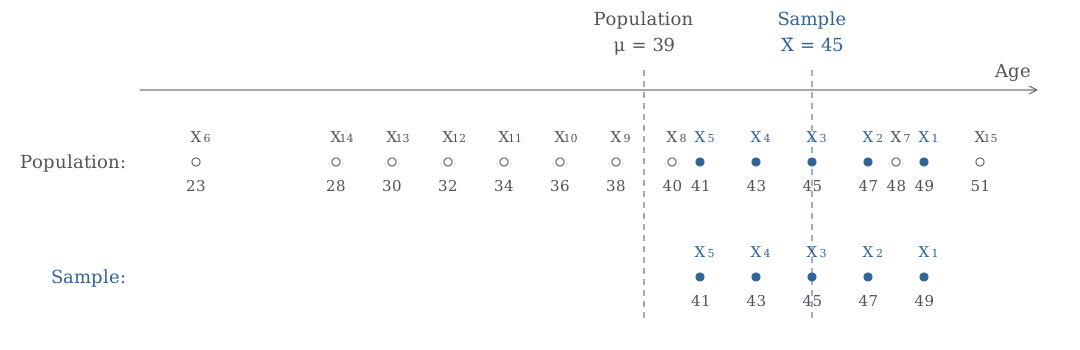
The population’s average age \(\mu\) is 39, and the ages are quite spread out. Now that we have sampled \((X_1,\ldots,X_5)\), we can naturally look at how far each person in our sample is from the true population mean:

\[ \begin{pmatrix} X_1-\mu\\ X_2-\mu\\ \vdots\\ X_5-\mu \end{pmatrix} \xrightarrow{\text{square, then average}} \frac{(X_1-\mu)^2+\cdots+(X_5-\mu)^2}{5}, \]

and use this to estimate the population variance \(\sigma^2\). This makes perfect sense: if we knew \(\mu\), dividing by \(n\) (five here) would be absolutely fine.

But here’s the trouble: we don’t know \(\mu\)! It’s the mean of all one million people, after all. So a natural thought is: we’re already using \(\bar X\) to estimate \(\mu\), so why not replace \(\mu\) with \(\bar X\) here too? That gives us our first step:

\[ \frac{1}{n}\sum_{i=1}^{n}(X_i-\mu)^2 \;\xrightarrow[\text{replace }\mu\text{ with }\bar X]{\text{Revision}}\; \underset{\star}{\underline{\frac{1}{n}\sum_{i=1}^{n}(X_i-\bar X)^2}}. \]

A small problem has quietly slipped in. We wanted to measure “how far the sample is from the population’s average age \(\mu\).” But \(\bar X\) isn’t the population’s centre: it is chosen after seeing our sample \(X_1,\ldots,X_5\). In our example, \(\bar X=45\). Look back at the picture: it’s pretty close to the five sampled people, isn’t it? It makes us think, “Hmm, these people—the solid blue dots ●—don’t seem all that spread out.” Yet in this example, the population, including the hollow grey dots ○, is much more spread out than our sample.

So think of it this way: the true mean \(\mu\) stays put, while the sample mean \(\bar X\) “chases after our sample.” If we happen to sample a younger group today, \(\bar X\) moves towards the younger ages. If we happen to sample an older group tomorrow, \(\bar X\) moves towards the older ages instead. So using \(\underline{\star}\) to estimate the population’s spread tends to underestimate it, on average. This brings us to the next step:

\[ \underset{\star}{\underline{\frac{1}{n}\sum_{i=1}^{n}(X_i-\bar X)^2}} \;\xrightarrow[\text{divide by }n-1\text{ instead}]{\text{Revision}}\; \frac{1}{n-1}\sum_{i=1}^{n}(X_i-\bar X)^2. \]

For our five-person sample, we go from dividing by five to dividing by four. This makes the estimate a little bigger, to offset the underestimation caused by using \(\bar X\)—and that answers our opening question.

---

A small remark. How much does \(\underline{\star}\) underestimate the variance, exactly? We can describe this using the mathematical language of ST2131: expectation. With independent, identically distributed observations of finite variance, a little calculation gives:

\[ \begin{aligned} E\!\left[\underline{\star}\right] &=E\!\left[\frac{1}{n}\sum_{i=1}^{n}(X_i-\bar X)^2\right]\\ &=\frac{1}{n}\sum_{i=1}^{n}E\!\left[(X_i-\bar X)^2\right]\\ &=\frac{1}{n}\sum_{i=1}^{n}E\!\left[\big[(X_i-\mu)+(\mu-\bar X)\big]^2\right]\\ &=\cdots=\frac{n-1}{n}\times\sigma^2. \end{aligned} \]

Don’t worry—try expanding the square, treating each expression in parentheses as one piece!

This means that if we repeat the “sample just five people” experiment many times, \(\underline{\star}\) averages out to \(4/5=80\%\) of the true variance. If we repeat the “sample 100 people” experiment, it averages out to \(99/100=99\%\). So as the sample size gets larger, dividing by \(n\) or \(n-1\) makes less and less difference.

---

Let’s try sampling!

Choose a population distribution and a sample size, then draw ten samples. Every population below has variance 100, so we can compare the two estimates on equal footing even when the shapes look very different.

This idea does not stop here. In ST3131, when we study regression, we will meet similar variance estimates where the sum of squares is divided by (n-2) or (n-p). If you come across them and would like to see how the same idea carries over, take a look at Why (n-2) in Regression Variance?.